gregers kjerulf dubrow - r to Tableau, then show it in Quarto

allison horst r artwork — r plays nicely with other outputs

tl/dr - I’m trying to show I have some Tableau skills to go with my r skills to help my chances at employment (hint-hint).

Introduction

Tableau has long been on my list to add to my data analysis skillset. I’ve tried in fits and starts over the years, but hadn’t been able to sustain it due to work and life.

I had hoped to get to it in the fall, after my CIEE contract ended and I knew I’d be without work for a bit. But four Danish classes a week and doing a few r projects for the blog took up some time. Then in late December I was on the wrong end of a bike-car collision (more on that later in bike and healthcare-related posts), and after I got back from 2 weeks in the hospital and started to feel better, I decided it was time to take it on.

I started by replicating the superstore data exec dashboard, then wanted to do an original project. Initially the idea was to do a dashboard with some other data, and see if I could embed it in a blog post using Quarto. While working on that I somehow got the idea I wanted to make the visualisation be a paramterized user-choice analysis.

I wasn’t nuts about the older data suggested by Tableau, and given I’m using the free Tableau Public product and I don’t yet know how to connect to data and clean in Tableau, I decided on this analysis workflow for this 1st project:

Use r to source and clean the data, export to CSV.
Build a visualisation in Tableau, on-line
Write a blog post wherein I attempt to embed the Tableau viz.

I’ve seen the embedding done in Jon Boeckenstedt’s college enrollment trends blog (I think he uses blogger) and hope it works here. (spoiler alert…it does)

Getting & cleaning some data

So first, let’s source and clean some data. I’ve long wanted to try the worldfootballr package, so we’ll use that to get data for the English Premier League’s 2022-23 season. I ultimately want a dataset with total points and goals, expected points and goals, actual minus expected, and these items also for home and away matches.

code to get and clean the data and write to csv

### template for r analysis work. save as w/ appropriate name to project directory

library(tidyverse) # to do tidyverse things
library(tidylog) # to get a log of what's happening to the data
library(janitor) # tools for data cleaning

# EDA tools
library(DataExplorer)
library(explore)
library(skimr)

# some custom functions
source("~/Data/r/basic functions.R")

# get 2022-23 match result data from understat via worldfootballr
epl_results2223 <- understat_league_match_results(league = "EPL", season_start_year = 2022) %>%
    select(-isResult)

# because of the way the data comes, need to separate out into home and away dfs
epl_2223_byteam_home <- epl_results2223 %>%
    select(home_team, home_goals, away_goals, home_xG, away_xG, forecast_win, forecast_draw, forecast_loss) %>%
    group_by(home_team) %>%
    mutate(ga_home = away_goals) %>%
    mutate(xga_home = away_xG) %>%
    # actual points using match result
    mutate(points_home = case_when(home_goals > away_goals ~ 3,
                                                                 home_goals < away_goals ~ 0,
                                                                 home_goals == away_goals ~ 1)) %>%
    # expected points using match probability...it's a crude measure but works for our purposes
    mutate(points_exp_home = case_when(((forecast_win > forecast_draw) & (forecast_win > forecast_loss)) ~ 3,
                                                                         ((forecast_draw > forecast_win) & (forecast_draw > forecast_loss)) ~ 1,
                                                                         TRUE ~ 0)) %>%
    # create sum for each column and bind that row to the df
    mutate(Total = rowSums(across(where(is.numeric)))) %>%
    bind_rows(summarize(., description.y = "Total", across(where(is.numeric), sum))) %>%
    # select only the row with totals
    filter(description.y == "Total") %>%
    # create a few more variables
    mutate(goals_minus_xg_home = home_goals - home_xG) %>%
    mutate(ga_minus_xga_home = ga_home - xga_home) %>%
    mutate(points_minus_points_exp_home = points_home - points_exp_home) %>%
    ungroup() %>%
    select(team = home_team, goals_home = home_goals, xg_home = home_xG, goals_minus_xg_home,
                 ga_home, xga_home, ga_minus_xga_home,
                 points_home, points_exp_home, points_minus_points_exp_home)

# the same steps but for away team...note the differences in coding actual & expected points
epl_2223_byteam_away <- epl_results2223 %>%
    select(away_team, home_goals, away_goals, away_xG, home_xG, forecast_win, forecast_draw, forecast_loss) %>%
    group_by(away_team) %>%
    mutate(ga_away = home_goals) %>%
    mutate(xga_away = home_xG) %>%
    mutate(points_away = case_when(home_goals <  away_goals ~ 3,
                                                                 home_goals > away_goals ~ 0,
                                                                 home_goals == away_goals ~ 1)) %>%
    mutate(points_exp_away = case_when(((forecast_loss > forecast_draw) & (forecast_win < forecast_loss)) ~ 3,
                                                                         ((forecast_draw > forecast_win) & (forecast_draw > forecast_loss)) ~ 1,
                                                                         TRUE ~ 0)) %>%
    mutate(Total = rowSums(across(where(is.numeric)))) %>%
    bind_rows(summarize(., description.y = "Total", across(where(is.numeric), sum))) %>%
    filter(description.y == "Total") %>%
    mutate(goals_minus_xg_away = away_goals - away_xG) %>%
    mutate(ga_minus_xga_away = ga_away - xga_away) %>%
    mutate(points_minus_points_exp_away = points_away - points_exp_away) %>%
    ungroup() %>%
    select(team = away_team, goals_away = away_goals, xg_away = away_xG, goals_minus_xg_away,
                 ga_away, xga_away, ga_minus_xga_away,
                 points_away, points_exp_away, points_minus_points_exp_away)

## bring in league table info...note, this is from FB Ref, and XG formula is different from understat. FB Ref uses opta,
 ## understat has their own formula. we'll use the understat xG in the final dataset
epltable_2223 <- fb_season_team_stats(country = "ENG", gender = "M", season_end_year = "2023", tier = "1st",
                                                                            stat_type = "league_table") %>%
    rename(team = Squad) %>%
    # fix a few team names that FBRef has in a different format
    mutate(team = case_when(team == "Nott'ham Forest" ~ "Nottingham Forest",
                                                    team == "Manchester Utd" ~ "Manchester United",
                                                    team == "Newcastle Utd" ~ "Newcastle United",
                                                    TRUE ~ team))

## merge all together, fixing team names, creating new fields.
epl_2223_byteam_all <- epl_2223_byteam_home %>%
    merge(epl_2223_byteam_away) %>%
    mutate(team = case_when(team == "Wolverhampton Wanderers" ~ "Wolves",
                                                     team == "Leeds" ~ "Leeds United",
                                                     team == "Leicester" ~ "Leicester City",
                                                     TRUE ~ team)) %>%
    merge(epltable_2223) %>%
    mutate(goals_total = goals_home + goals_away) %>%
    mutate(xg_total = xg_home + xg_away) %>%
    mutate(goals_minus_xg_total = goals_total - xg_total) %>%
    mutate(ga_total = ga_home + ga_away) %>%
    mutate(xga_total = xga_home + xga_away) %>%
    mutate(ga_minus_xga_total = ga_total - xga_total) %>%
    mutate(points_total = points_home + points_away) %>%
    mutate(points_exp_total = points_exp_home + points_exp_away) %>%
    mutate(points_minus_points_exp_total = points_total - points_exp_total) %>%
    select(team, rank = Rk, W:L, Pts, Pts.MP, points_total, points_home, points_away,
                 points_exp_total, points_exp_home, points_exp_away,
                 points_minus_points_exp_total, points_minus_points_exp_home, points_minus_points_exp_away,
                 goals_total, goals_home, goals_away,
                 xg_total, xg_home, xg_away, goals_minus_xg_total, goals_minus_xg_home, goals_minus_xg_away,
                 ga_total, ga_home, ga_away, xga_total, xga_home, xga_away, ga_minus_xga_total,
                 GF:GD, xG:xGD.90)

# write to a CSV we'll import to Tableau
write_csv(epl_2223_byteam_all, "~/Data/football data files/epl_2223_byteam.csv")

Embed the Tableau workbook

Ok…CSV written, uploaded to the Tableau workbook. I used this guide to build the parameters, and used other tips from the superstore exec summary how-to vids.

To embed the Tableau workbook here I copied the embed code and placed in a code chunk with {=html} after the first three tick marks, then the embed code below the html tag.

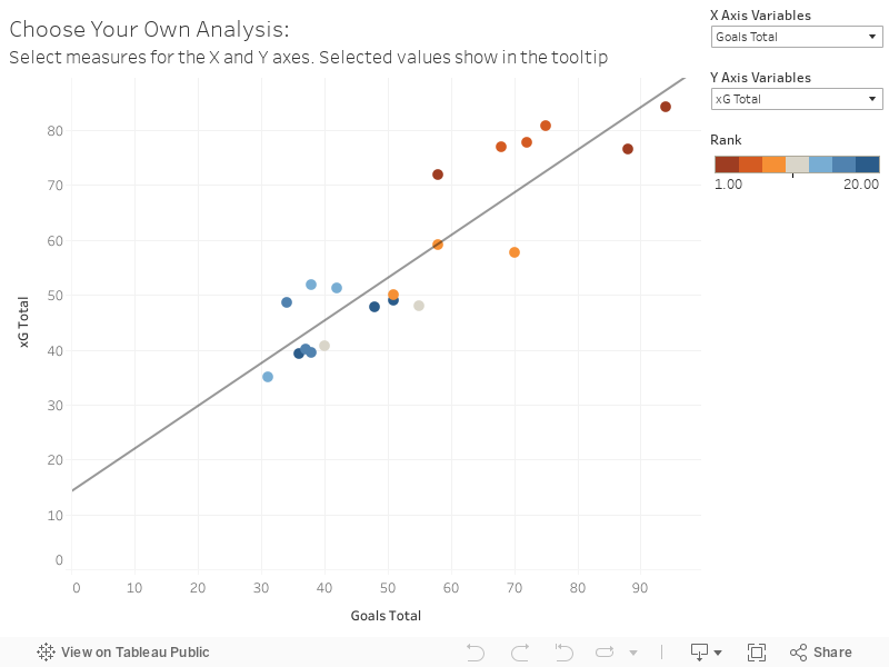
You can play with the data here on this page or you can go to the book on my Tableau profile. If the data tell any story it’s that teams who maximize chances (convert xG, expected goals) to actual goals, have a better chance of turning expected points into actual points. Not groundbreaking analysis to be sure.

It’s not necessarily a final version - there are more variables to add to expand user choice, but it’s enough now to get the main point, which was parameterized user choice.

More to Tableau visualisations to come as I get more familiar with it and want to try new chart types and visualisations.

But hoooray, I proved the concept! Injury-induced downtime FTW!